Some fluids need progressively lesser force to increase velocity...
If you have ever been part of the whole drilling project starting from planning to execution to completion to handover, you would be aware that there all lots of uncertainties that occur which are either beyond your control or wasn’t considered during the planning stage. This affects the timeline of the project and the consequences of those are well known in the industry. Therefore, there was a need for to quantify these uncertainties and put it on paper for those involved in the decision-making process to understand the extent of variation in the estimate of the Drilling Time.
For example, the Rate of Penetration (ROP) while drilling varies based on the bit type, other drilling parameters and the formation properties. These properties are not uniform. The ROP therefore varies based on the depth and these factors and is not a constant. Similarly, there would be uncertainties in the times for all the operations involved in the drilling campaign.
Monte carlo modelling helps in quantifying these uncertainties backed up by relevant and sound data. Instead of using a single estimate of time, monte carlo method uses probabilistic methods to forecast the time for each operation and in total for the whole well.
The origins and history of the Monte Carlo method are not discussed here. Many sources can be found online if the reader is interested. We will merely discuss about how it is used in drilling time estimates. Before we dive in, the MC method is basically a method in which multiple random experiments and simulations are performed. Ideally around a thousand simulations are performed and is more than enough in the case we are dealing with. The basic idea to run multiple experiments with the system of interest. In this case we simulate drilling thousand wells. Ideally the best method to run the experiment is to actually drill the well a thousand times and then get the time taken for each activity. Now, this is totally impractical and doesn’t serve our requirements. Instead, for each drilling activity we randomly sample a specific value of time from an appropriate probability distribution and then calculate the total time taken for the well. Do this a thousand times and we have a Monte Carlo simulation of the well. With this result, we can determine the minimum, the maximum and the average time it takes to drill the well and determine the variability (which is the uncertainty).
First thing’s first, you need to list down all the activities that are going to take place in the well. Now, for each activity you need to identify the parameters that affect its duration. For example, as stated before, the drilling time is affected by the ROP. For tripping time, it would be the tripping speed and so on. There are some activities that won’t have any direct parameters such as Nipple Up BOP or Wellhead Installation. For these activities you simple the time taken to complete the activity would be the parameter to model.
This step is the most crucial one because the model is sensitive to the type of distribution. If an erroneous distribution is selected for the parameter, then model would produce an error in the estimate. There are many types of distributions that are typically considered. The most common being:
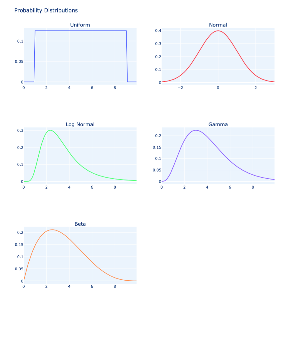
Each of these distributions will have its own set of parameters that describe the probability curve. Either an educated guess can be used to set these parameters or you can use the actual time taken in offset wells to get the best fit distribution to get the required parameters. The latter method is more accurate but is tedious and would be close to impossible to do if there isn’t any well data - for each parameter at least 30 data points are required as a general rule of thumb to get an accurate description of the distribution.
This is the best part. You can now run the simulation as many times as you want. Running the simulation a thousand times would be suitable enough. So how does the simulation work?
For each run of the simulation, the model will randomly sample a value from the probability distribution for each activity. This simulates one random outcome for the activities' duration. The sum of the duration for each activity will give you the total well time. This is one random outcome for the well. Do this a thousand times and you get a thousand random outcomes for the well time estimate.
Now you will have multiple time estimates for the well. You have the overall probability distribution for the total well time which is the final goal required. A range of possible time estimates for the well can be identified inside a confidence interval. For example we can say that there is a 10% chance or probability that the “well would take less than or equal 25 days to drill and a 90% change it will exceed 25 days”. Read the statement again and you will see the words less than or equal or Exceeding. For the same case, the usual interpretation which is unfortunately understood by many is that “10 out of 1000 wells drilled with take 25 days”. This statement doesn’t make any sense for the fact that the same well is not going to be drilled 1000 times and moreover that’s not what a probability distribution models in the first place.
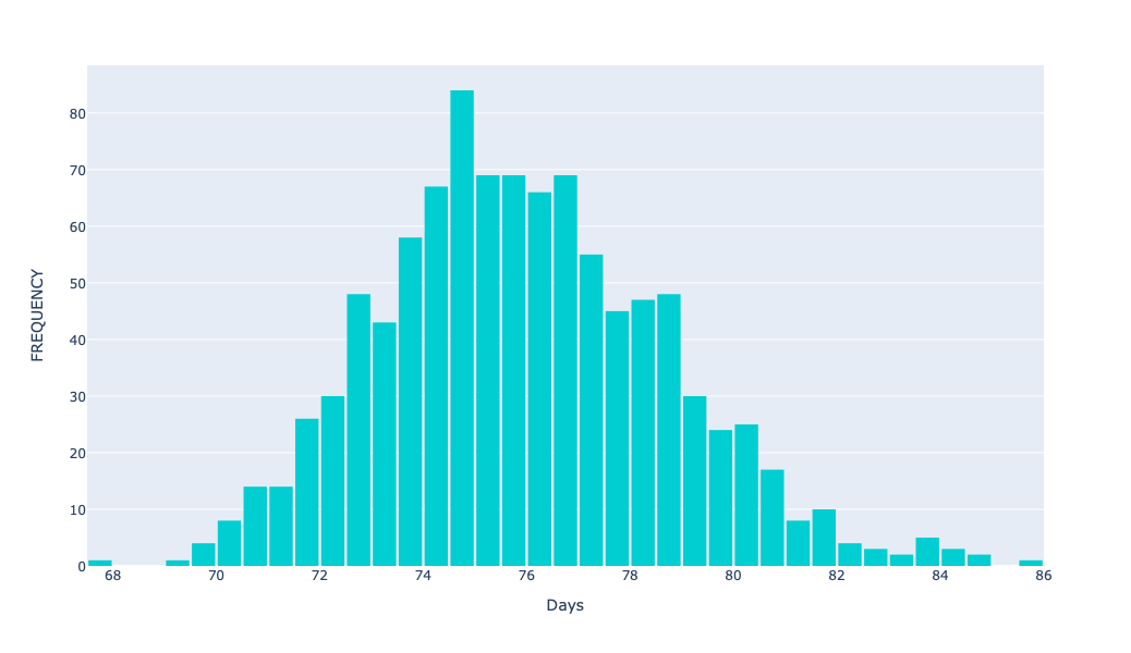
So now we have a range of possible outcomes for the total well time. Using this information, a histogram can be drawn up as shown here, which describes the distribution in terms of frequency of recurrence. This can be converted to a probabilistic data but will have the same shape and spread. Only the Y axis would change where instead of Frequency you would have the probabilities.
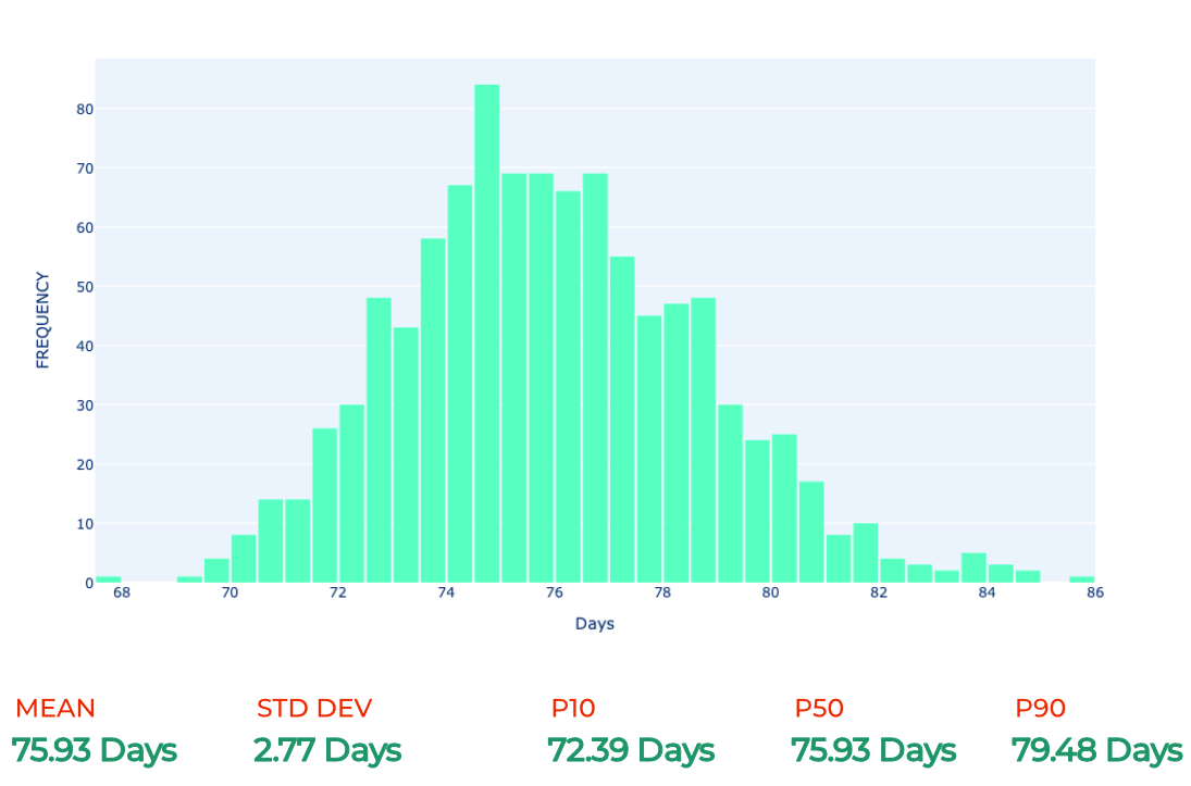
Therefore, the total well time will also have distribution parameters such as mean, median, mode, variance and standard deviation (among others). Although this is crucial information for a Q&A Engineer, for a drilling engineer, well manager or other management professionals, their interests lie in simply the variation in time for the whole well.
A simplified result which is more useful is to have confidence interval for time within which the well can be drilled. The usual standards are to have the 10%, 50% and 90% confidence interval. This is termed as the P10, P50 and P90 estimates as shown below. Some operators also prefer to have P30 and P70 times (30% and 70% Confidence Intervals). The more inquisitive reader would have asked then question “Would there be 0% and 100% confidence intervals, or P0 and P100 estimates?” and the answer is “Yes”. The P0 and P100 times are simply the minimum and maximum time obtained from the simulated well time distribution respectively. This brings the discussion again to the interpretation. When you consider P0 time, it does not mean that 0% of the wells take – 68 days in this case - to drill (Again, the statement makes no sense). It actually means that the time taken to drill the well is definitely more than 68 days. The same interpretation goes for all the other Pt times. P100 would mean that the well time would never exceed the P100 estimate - 86 days here - and rather it would less than the P100 estimate.
Once the Probabilistic Estimates for the total well time is ready, now the Time vs Depth chart will be prepared like the one here.
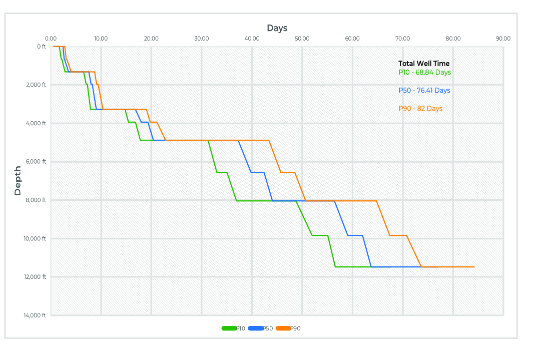
The Time vs Depth chart is the final result of this process. Although it can't be observed directly here, the Time vs Depth chart here is actually the cumulative activity time distribution at every depth.
P10, P50 and P90 are the usually represented time estimates in the chart, but you can also include the Minimum and Maximum time estimates as well. Moreover many Operators include the P30 and P70 time estimates.
As you can see, the entire process requires time, computational effort and more importantly accurate assumptions and distribution of your parameters. Given all of these requirements, allows us to understand uncertainty and risks.
This article describes briefly the workflow of Monte Carlo in Drilling Time Estimates. The internal working and statistical analyses involved are detailed. To understand the statistical methods used, a complete study on Random Processes and Applied Probability is required. There are many references and online materials available to understand the basics of probability.
Finally, talking about risks, there are methods to include unforeseen risks in the time estimate such as Stuck Pipe, Loss Circulation, Well Control incidents etc., and other Non-Productive Times. These will be discussed in another article in the series.
Sri Krishna is a drilling engineer and is the co-founder of iDrilling Technologies. He has experience in well engineering and implements modern data science methods to analyze well data and do the well design.
All author posts
Some fluids need progressively lesser force to increase velocity...